IEEE 754 Floating Point Numbers
(Note: strictly speaking these are the interchange formats, which specify the meaning of particular bit patterns)
To specify a format
- # exponent bits
- # significand / mantissa / fractional bits
- base
(also a bias, though this isn’t part of the format)
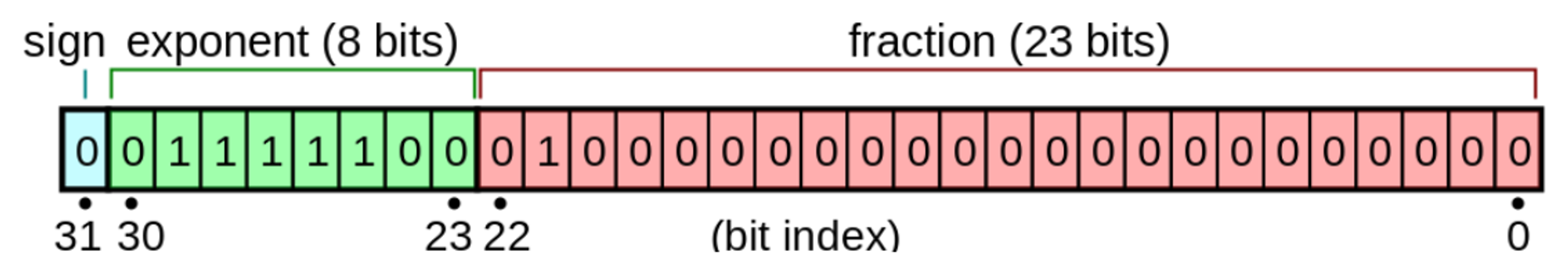
To specify a number in a given format
- sign bit
- exponent bits
- significand / mantissa / fractional bits
Interpretation of fp number
Given: sign bit ; exponent bits , fractional bits ; base ; bias :
Special values
If all exponent bits = 1 and significand field = 0: infinity
If all exponent bits = 1 and significand field != 0: NaN
If all exponent bits = 0: subnormal number ➡️ leading bit of significand now implicitly zero, allowing even smaller (in absolute terms) numbers
Specific Formats
Formats (1)
Significand bits sometimes reported as 1+ ⬆️ values, as they include implicit bit
Base = 2, bias = for all.
Introduction
How should we represent numbers on a computer? This turns out to be one of the most important questions in building performant ML systems.
The consistent breakthroughs from ever larger models indicates that scale is currently the most important factor in improving model performance (see the Bitter Lesson). This leads to the question: what’s the most important factor underlying scaling?
In the days of Moore’s Law it would be semiconductor transistor density. But Moore’s Law is over. In fact, since the emergence of GPUs for ML in 2012 the primary speedup has been from numerics () rather than transistor density ().
This improved performance, combined with learning how to distribute training over multiple chips, are key factors in the current trend of massive scaling.
It’s likely that future models will continue to try and exploit this, pushing numerics to near their limit. So having a clear understanding of this area, the trade-offs involved, and how numerical formats interplay with algorithms, is key to understanding current and future ML systems.
Integer representations
Starting with the simple case, let’s examine integer representations. This is not especially important for ML systems, but will lay the groundwork for real-valued number formats, which are.
An unsigned integer is simply a binary number. Some complexity in introduced when representing signed integers, which we’ll explore below:
Sign-magnitude
Think of this as the “human” approach to representing integers.
The most-significant bit is a sign bit (i.e. ‘+’ or ‘-’) and the other seven bits are simply the number that follows, represented in binary.
This has some downsides however:
- There are two ways of representing 0
- A consequence of this is that our range is only values
- Arithmetic can be fiddly when handling calculations where the sign bit changes
The following methods address these issues:
One’s complement
This format is the same as sign-magnitude, except that when the most-significant bit is set the remaining bits are interpreted as having been inverted.
This makes arithmetic simpler when dealing with the sign bit.
However it still has the downside of two 0 representations.
Two’s complement
This is the scheme implemented in most modern integer representations.
It is the same as one’s complement, except that when a positive sign bit is seen we now interpret it as having flipped the bits and added 1.
This scheme has a second interpretation: that all bits are now “valid”, but the most-significant bit represents (whereas it would usually represent ).
This representation has the benefit of a single 0 representation, and arithmetic is still easy to implement.
Offset binary
We’ll cover one final representation here, because it has links to the floating-point representations that will follow.
The offset binary method simply defines an offset value (typically ), and we interpret the bits like an unsigned integer, minus .
This only has a single 0 representation, though unlike in the other schemes, here the number zero is not represented by a series of 0s, but by the number .
Real number representations
With integers we implicitly assumed that the ideal approach was to represent a set of adjacent numbers.
However, we could instead have opted for a representation that covered a wider range of numbers, but in a sparse way. This is the approach we will have to take for real-valued numbers.
Fixed-point representations
This is the most basic approach to representing real numbers. We interpret our bits as an unsigned integer, and assume an implicit scale factor by which they are multiplied.
For example, given a scale factor of , the bits (i.e. 10) would give a representation of .
We also have a leading sign bit, which operates in the expected way (i.e. the sign-magnitude system above).
We use the term fixed-point to indicate that in the binary representation of this scheme, the floating point never moves. In the above case we end up with , and the point stays in the middle regardless of the bit pattern we choose.
Depending on the scale factor we choose, we can represent any range (that’s a power of 2).
The distribution of values