Intro
A lot of sparsity research has been in the limited data domain. Here models can saturate and can’t do any better. In this setting sparsity can look great, but what about the more general non-data-limited regime?
This is not well studied. Paper attempts to do so for lang and vision transformers, fitting scaling law, predicting loss given:
- Number of non-0 params
- Sparsity level
- Tokens seen
Setup
Sparsity research has often focussed on the data-constrained case, where models can saturate and the benefits of sparsity are substantial. Here they focus on the more important unlimited-data regime, in which it has never been shown sparse models can win in a fair comparison.
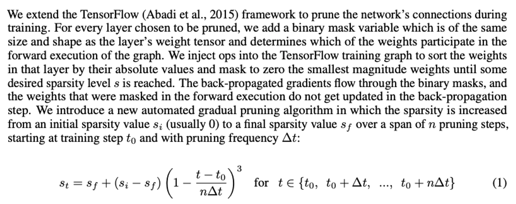
How do they sparsify? “via gradual magnitude pruning (Zhu & Gupta, 2017), using a cubic schedule starting at 25% of training and ending at 75%” - clip from that paper is below (it’s exactly what you expect)
Deriving the scaling law
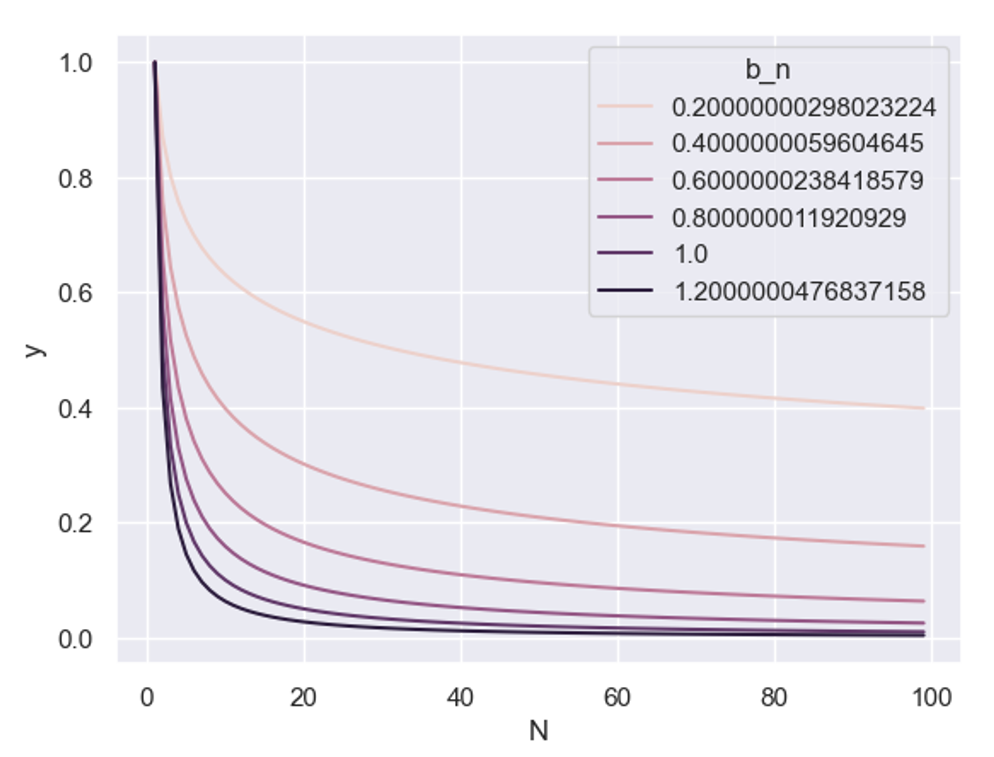
They plot these curves:
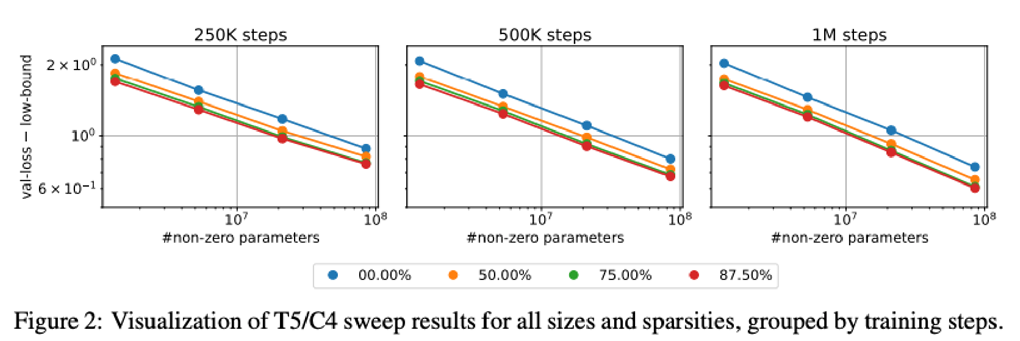
Then look at the shapes and characterise what’s going on as:
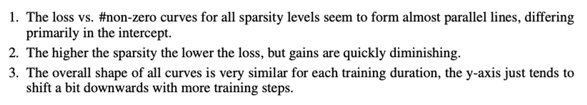
Given these features, this suggests the following form:
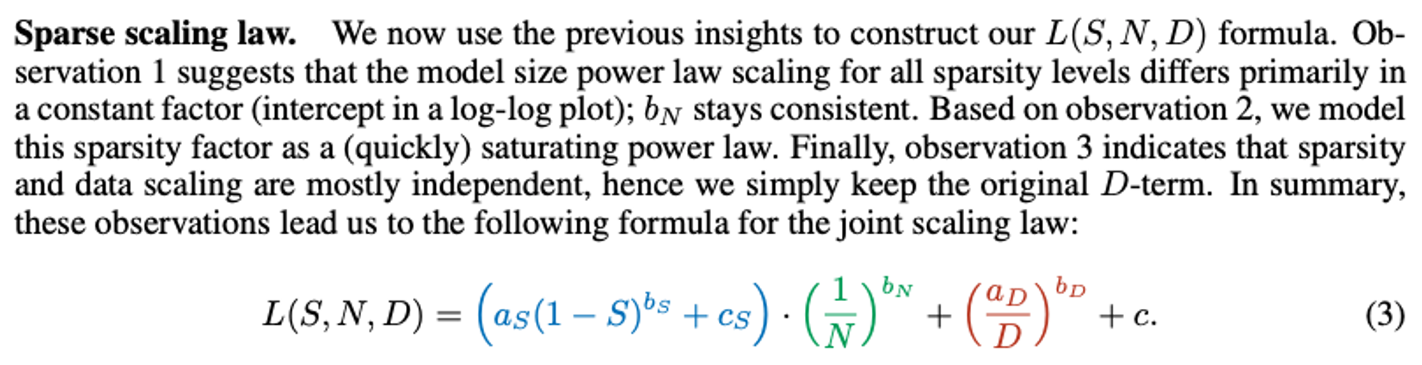
Scaling Law Formulation
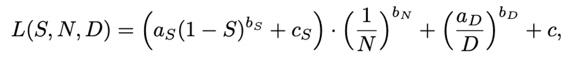
Can we get some intuition for this?
For comparison, recall the “standard” scaling laws maths:

The power terms drop off like a 1/x curve, with the exponent controlling how hard the drop-off is. The larger the exponent, the “more powerful” that term is in making the loss fall.
The term is just a multiplier on the “D” part as a whole, also controlling where it starts.
The first “S” part could be seen as another power-law, e.g.
Where is the inverse density. For this term, full density (S=0) is 1, and as the tensor tends to emptiness (S=1) the ID tends to infinity. This acts a lot like terms such as number of params and data, so it’s quite nice.
The constants give a lower bound - the main for the loss as a whole (irreducible loss), and for how much sparsity can help you. This effectively clips it’s max effectiveness.
The fact that it’s multiplied by the params loss I suppose relates to the fact that it has a direct relationship with the param count??
The Results
Given all this maths, they can then fit the params to their data.
Extrapolation
To validate it’s doing something sensible, they train one much larger model (lower loss) and extrapolate to it. Looks pretty good!

Optimal sparsity
We can do some maths to calculate the cost C for dataset D in terms of a) dense (regular) flops, and also b) sparse (only compute non-zeros) flops. With this calculated, we can substitute it into our loss to get it in terms of the (S, N, C) triple.
We then differentiate wrt. to S and set the result to zero. This can be solved to find the sparsity S that minimises the loss for a given (N, C) pair.
Thus for every point on an NxC grid we have some value for S that is optimal. There are lines through this grid where S doesn’t change (i.e. where the optimal sparsity is consistent). These are “iso-contours” - we can plot them for a few different values of S:
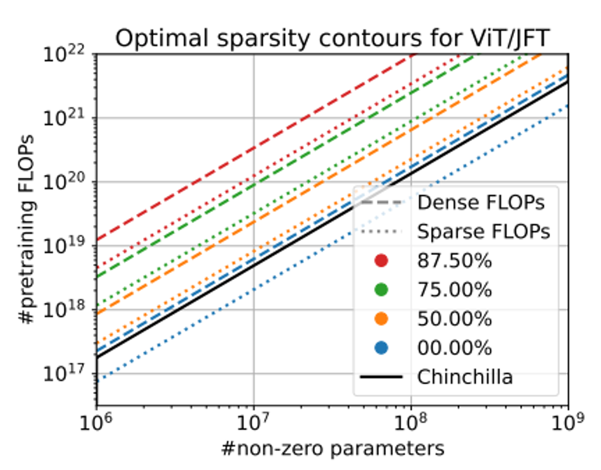
Note that because we had two different types of flops above, we have two different equations for optimal sparsity. These correspond to the two different style iso-contours above.
I think that everything to the bottom right of the 0% lines is also implicitly 0%=optimal.
Conclusions from optimal sparsity
The key take-away from these results is that as one trains significantly longer than Chinchilla (dense compute optimal), more and more sparse models start to become optimal in terms of loss for the same number of non-zero parameters.
Practically this means that if you e.g. train a ViT for 2x longer than the chinchilla optimal FLOPs, you should use 50% sparsity.
Note though that this is in terms of sparse flops, which effectively assumes you can do sparse compute with no drop in throughput.
It also kinda assumes that you couldn’t just train a larger ViT, so you’re memory bottlenecked.
Other conclusions:
- Sparsity affects each model size in a similar way - as a multiplicative constant to the size scaling.
- Sparsity does not appear to interact significantly with dataset size
My take-aways:
- If you have a lot more memory than FLOPs (wrt. the Chinchilla limit), sparsity is unlikely to help you.
- If you have roughly the Chinchilla ratio, it may help a bit, though only at high density.
- As we start to use more FLOPs than Chinchilla recommends, the optimal density becomes lower. You need to train for a lot longer than recommended before very low-density models begin to make sense.
- All of this assumes you store weights sparsely.
- If you can leverage sparsity for compute (i.e. only compute on non-zero elements), the optimal density at a given point becomes lower (for ViT it roughly halves).
- Note that nothing here accounts for the overheads of sparse compute or memory access, so the “truly optimal” values are likely quite a bit higher.
Extensions
N:M Sparsity
Nvidia uses 2:4 (50% sparsity). They also explore other 50% and 75% schemes.
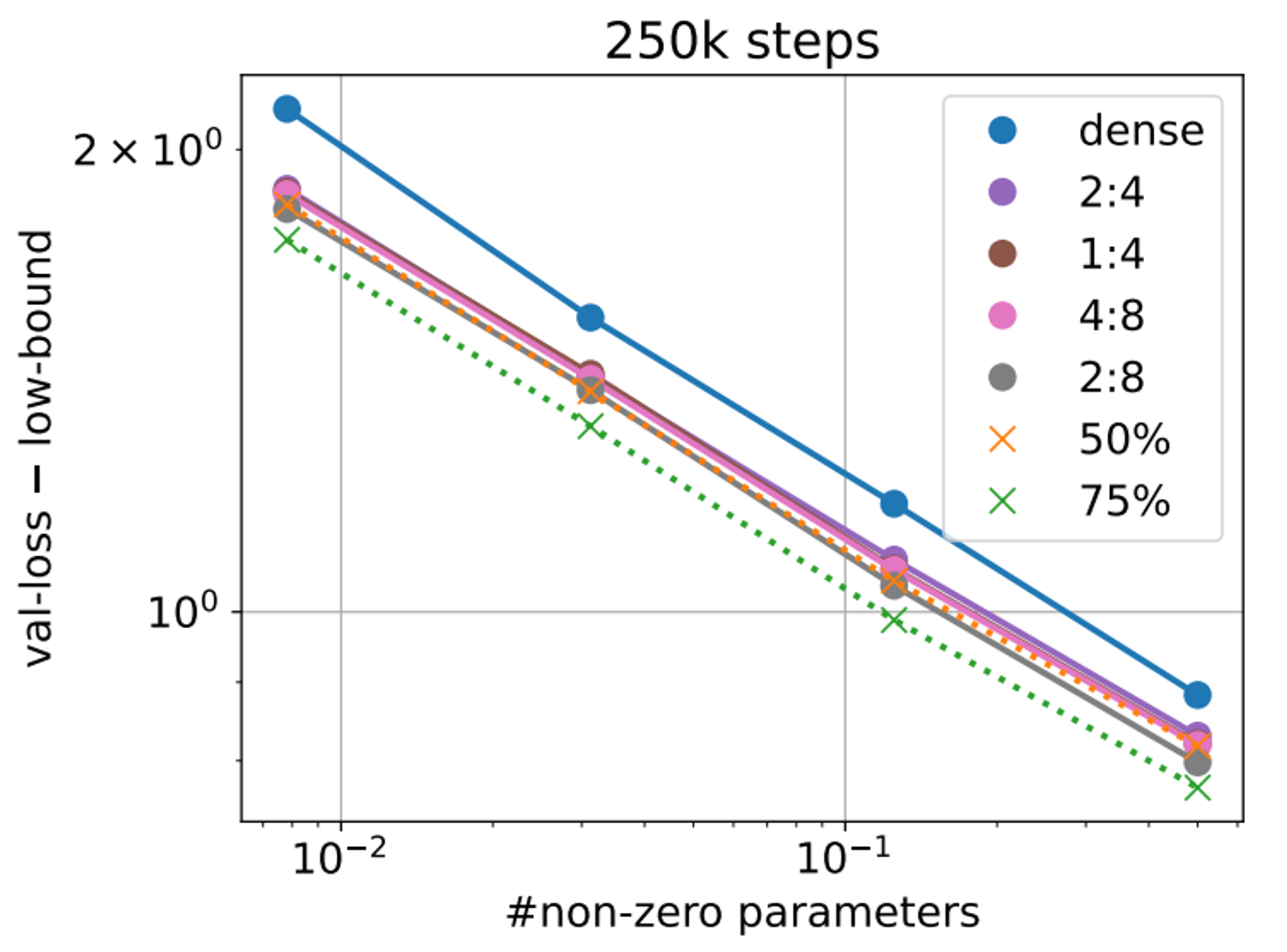
The takeaway here is that all the 50% schemes, including 2:4, get almost the performance of the unstructured 50% sparsity! The 75% schemes on the other hand are nowhere near - in fact they appear no better than the 50% structured sparsity. Why bother then.
What about storage for 2:4? If you can simply store the non-zero params and a little metadata (not sure), and get the full sparse flops throughput (I think so), then I think this is a (modest) winner looking at the 50% iso-contours on the main plot. But I feel I may be missing something…
Pruning Pre-trained Models
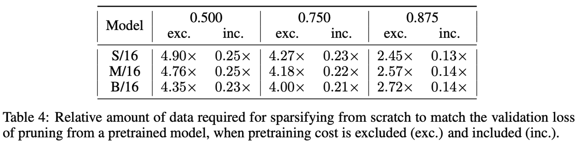
The way to read this table is:
- Assume I’ve done a 2-step process of pre-train a dense model, then sparsely fine tune it
- I now want to train up a loss-matched sparse model from scratch
- How much data does it take versus
- Step 2 - fine-tuning the dense model
- Step 1 + 2
Generally it takes a lot more data (e.g. 4x) than just step 2, but a lot less than the combined amount.
Conclusions:
- If you’re pre-training with a plan to later sparsify, best to just sparsity during training
- The benefit of having that pre-trained model decreases with sparsity (i.e. for v sparse you might just want to train sparsely from scratch). Rationale here is that the model is changing more with higher sparsity, so the pre-trained model is less helpful.
Discussion
Limitations
- Sparsity scheme is aimed for general, wide robustness. Could do better if more targetted
- Sparsifying for specific downstream application likely more effective than general sparsity
- Non-zero param count doesn’t account for difficulty of leveraging sparsity in practice
Overall conclusions
“
In particular, when training beyond
Chinchilla optimality, where simple dense training starts to run into diminishing returns, sparsity
can provide a clear alternative
note broken maths (why Simon look?)