Tensor Programs V

Paper Notes

Parameterization Tables

A parameterization is defined as

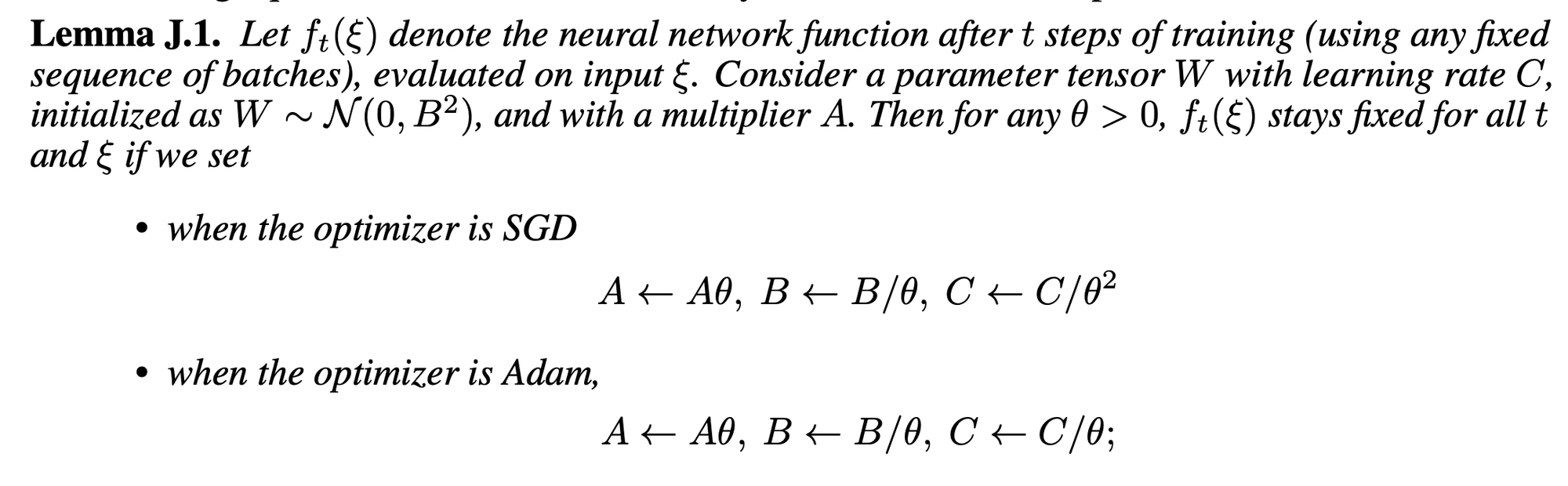
a rule for how to change hyperparameters when the widths of a neural network change, but note that it does not necessarily prescribes how to set the hyperparameters for any specific width

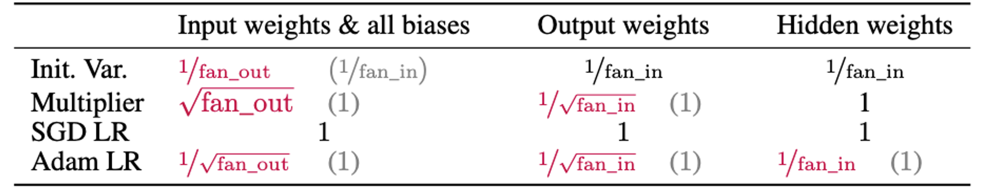
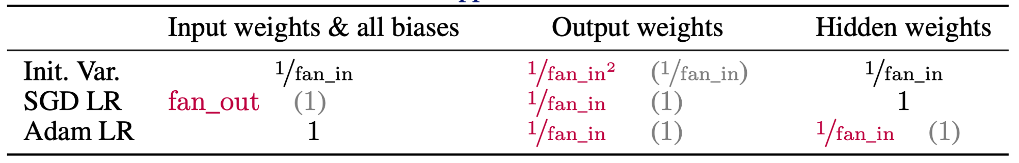
These three tables are apparently equivalent, just giving different trade-offs.

Main

Allows shared embeddings:

Directly follows from muP maths:

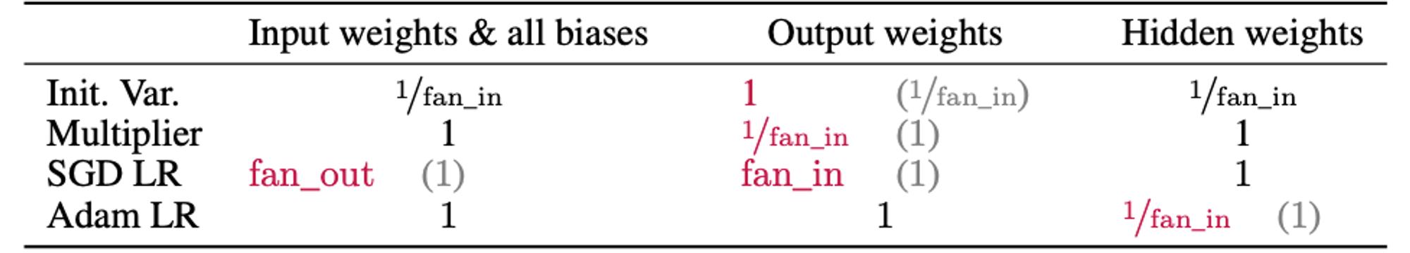
Input & output weights are defined as:

Those that map from a finite to infinite (i.e. scales with width) dimension.

E.g. transformer in & out projections

The method for jumping between the tables

(though there’s some extra slight of hand somewhere to get from col 1 of table 3 to the other two)

The above also means the following unit-scaling equivalent table is valid

ㅤ	Input w&b	Output weights	Hidden weights
Init Var	1	1	1
Multiplier	1/sqrt(fan_in)	1/fan_in	1/sqrt(fan_in)
SGD LR	fan_out * fan_in	fan_in	fan_in
Adam LR	sqrt(fan_in)	1	1/sqrt(fan_in)

(rule: *c, /sqrt(c), *c, *sqrt(c))

How does the first column of the 1st table map to the 3rd?

They just set fan_in = 1. This is justified as it’s a finite dimension. After that the table-transfer rule applies exactly.

Introduction

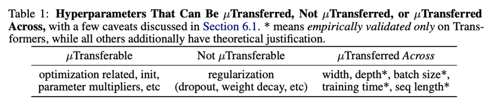
What can you mu-transfer?

In practice I guess the only one of the “mu-transferrable” ones that is always swept is the LR. Seems like this is really just for that HP. Some of these aren’t even typically considered HPs at all!

Interesting to see that a lot of the things that transfer aren’t theoretically justified. In a sense, technique is a lot more empirical than paper would suggest

Argument that muP is the unique parameterisation that allows HP transfer across width

Suggests US will have to change to fit muP, not vice versa.

Although given that most of their transfer stuff (see above) is actually empirical, maybe this is ok

muP has to be applied everywhere for it to work

In contrast to US, where you can (sort-of) pick-and-choose

The Defects of SP and How muP fixes them

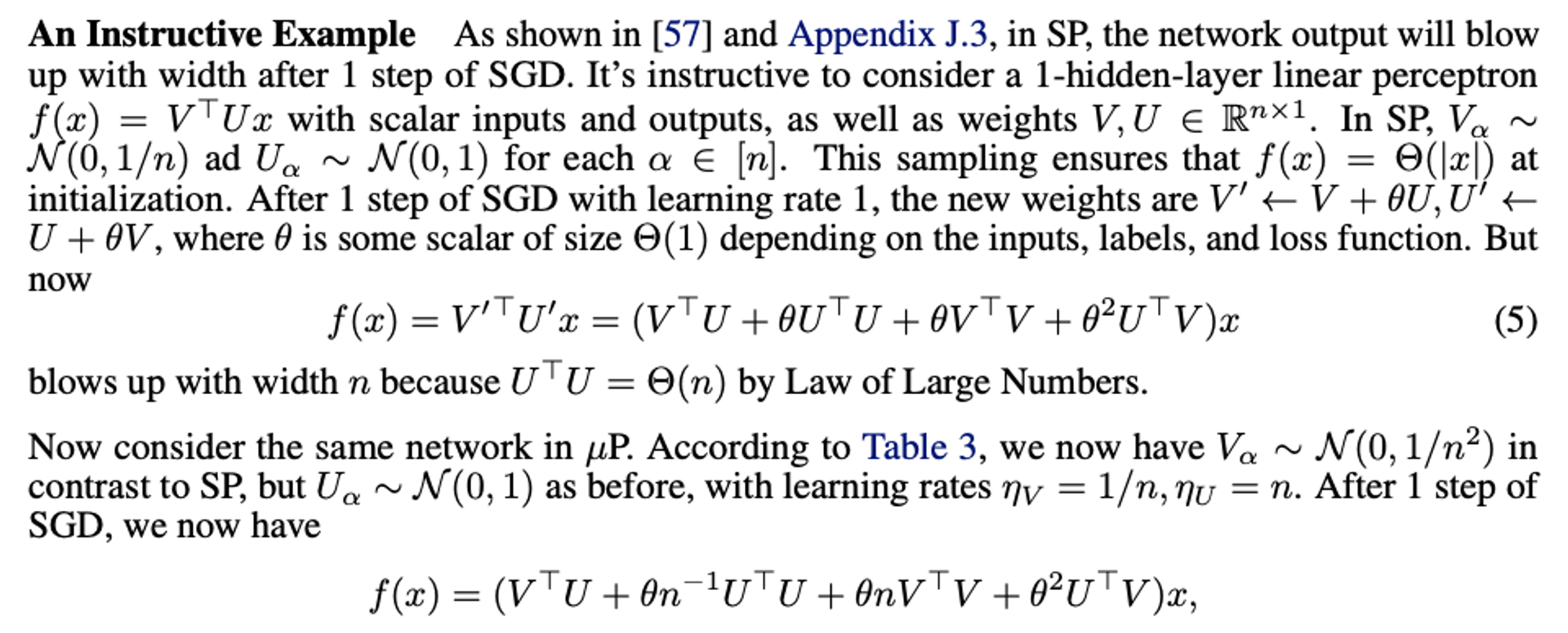
Instructive example

This is odd. I wrote the following to play around with this:


import torch
from math import sqrt
n = 2**20

## SP
V = torch.randn(n, 1) * 1/sqrt(n)
U = torch.randn(n, 1)

def f(U, V, x):
    return V.T @ (U * x)

print(f(U, V, 1))  # approx = 1

lr_v = 1
lr_u = 1
ϴ = torch.tensor([1.0])

def update(U, V, lr_v, lr_u, ϴ):
    
    V_ = V + lr_v * ϴ * U
    U_ = U + lr_u * ϴ * V
    return V_, U_

U, V = update(U, V, lr_v, lr_u, ϴ)

print(f(U, V, 1))  # approx = n

## muP

V = torch.randn(n, 1) * 1/n
U = torch.randn(n, 1)
lr_v = 1 / n
lr_u = n

print(f(U, V, 1))  # approx = 1/sqrt(n)

U, V = update(U, V, lr_v, lr_u, ϴ)

print(f(U, V, 1))  # approx = 1

U, V = update(U, V, lr_v, lr_u, ϴ)

print(f(U, V, 1))  # approx = n**2

A key criterion for their SP implementation is to get an O(1) output - muP doesn’t do this, why is that ok?

Their version does give something stable after 1 update, but then explodes after the 2nd update. Even with a smaller theta, the muP implementation explodes after the 2nd update.

Maybe the point is that it explodes at the same rate regardless of width … but I then tested this and it still doesn’t hold.

I’m not really sure what they’re trying to prove here. Unless my code is wrong?

What they say is that it “does not blow up with width” - and it’s true that after one step it will be stable across all widths. But this only works for one step, and the 0th-step output isn’t constant as a result

V & U becoming increasingly correlated here does seem to be an issue. I ran a quick test to check what happens when they aren’t and sure enough the update thing is fixed. This is probably a better reflection of reality, so muP isn’t as broken, but the output scale at initialisation is still weird…

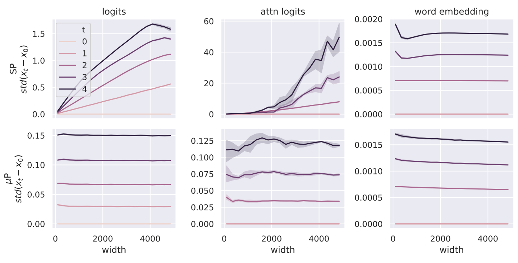
Key plot showing what muP fixes

The point is not that the scale remains stable across steps, it’s that the change doesn’t differ because of width.

Can just scaling down global lr with width fix this issue? Why do you need muP?

Some parts of the model (i.e. in-out layers) don’t depend on width, so this would effectively freeze those parts for large models

muP claims to outperform SP - how so?

In SP for large models we effectively have different update sizes for different parts of the model. The learning rate is then tuned for the most “explosive” parts of the model. Other parts then get scaled down and don’t learn properly (could this be why many models have stability issues at scale?)

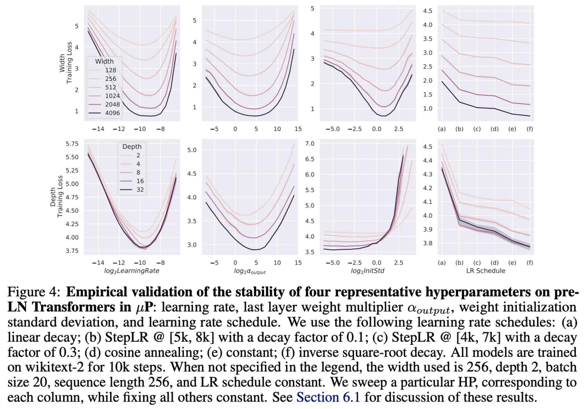
Results

What they run for the main sweep:

We sweep one of four HPs (learning rate, output weight multiplier, initialization standard deviation, and learning rate schedule) while fixing the others and sweeping along width and depth (with additional results in Fig. 19 on transfer across batch size, sequence length, and training time)

Models are tiny! We could replicate this on IPU quite easily.

The 32L model is only 25M. The 4096W model is 400M - big, but maybe we can just about squeeze on IPU with bs=1. Seq len is 256, so not too large 🤷 And if not we just stop at 2k. Remember that it doesn’t need to be fast.

Number of runs = num_hps * num_hp_options * (num_widths + num_depths + num_sls + num_train_times) * num_seeds ~= 4 * 10 * (6 + 5 + 5 + 5) = 4200 runs!

Some are BERT L size, but the base model is between BERT Tiny and BERT Mini - should be pretty fast

Transfer across depth (not theoretically justified) only works for preNorm, not postNorm

Are there results in the paper that show this?

An Intuitive Introduction to the Theory of Maximal Update Parametrisation

Setup: interesting point on sum of random variables

I’ve typically been assuming that . But if the mean is non-zero, we instead have

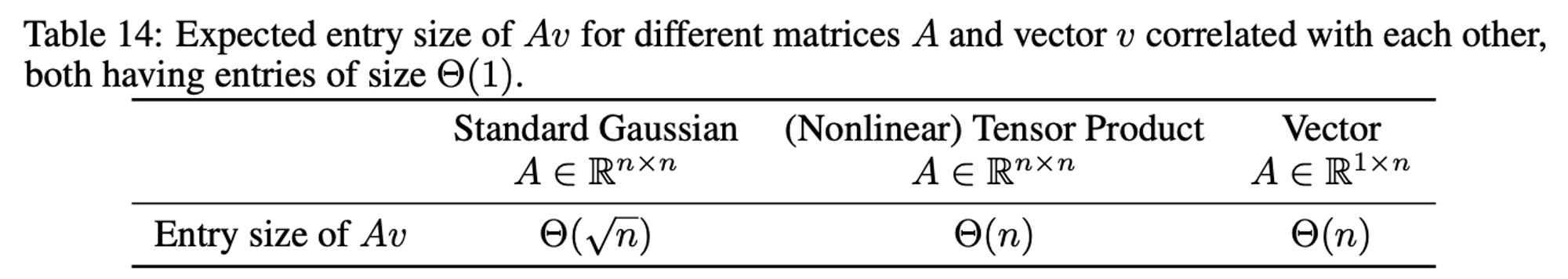
Three/four types of tensors considered:

iid normal

tensor product matrix (= sum of outer products, e.g. a grad_w (SGD update))

like 2. but more general → a nonlinear tensor product matrix (Adam update)

Expected entry size for

The paper explains that the gaussian case (col 1) is basically a weight-mul (in both the correlated and uncorrelated case!), col 2 is the weight update outer-product (sum). Not sure about the vector yet…

What it means for a vector to have -sized coordinates

They define this as:

I think this is the same as:

Which feels a bit more intuitive to me. Note also that the LHS is the std when the mean is zero - so this is (almost) just saying what the std is (e.g. )

Linear Tensor Product Matrix maths

This boils down to an analysis of the scale of

(they do a bit more - magnitude analysis and sum of outer products - but the outcome is the same)

Therefore they say the correct scaling factor for the weight update is . Our analysis would say ! The reason is correlation assumptions (see below)…

“in the general case v and x are correlated (as is generically the case during gradient descent, with A = ∆W for some weights W and x being the previous activations)”

Aaugh! We need to understand if they have some principled reason for this, or if it’s what we think…

Their conclusion for the Linear Tensor Product Matrix maths is that: is the right coordinate size for A

I was expecting this to imply a LR of 1/n (certainly for the hidden weights), but it isn’t … I’m assuming then that they “come out like this” in the network and don’t need correction. Will wait and see…

Nonlinear Tensor Product Matrix maths

This maths seems to basically be saying that the extra stuff Adam does with the gradient update doesn’t depend on the dims of the tensor (which is obvious! but anyway…) so therefore the SGD analysis holds for Adam as well.

They say “A has coordinate size and this is the unique scaling that leads to having coordinate size ”. So it sounds the same as above, except…

Their table gives 1/fan_in for the Adam LR rule!? Not getting this yet…

muP desideratum 1: Every (pre)activation vector in a network should have Θ(1)-sized coordinates

How does this compare to us? So our current target is

Where we generally assume that . This isn’t ideal actually, because for large this value can equal 1 and still give huge numerics issues. If we were to aim instead simply for:

This would solve that problem (and still in “natural units”, unlike variance-based targets).

This would then allow us to align with their criterion as well. For them “-sized coordinates” means:

Or equivalently:

Our target of is one particular case of this, so unit scaling satisfies their first desideratum (it doesn’t go the other way → one could have a large constant value which would be ok for muP, but bad for US numerics)

muP desideratum 2: Neural network output should be O(1)

They also add: “with desideratum 3, this means the network output should be Θ(1) after training (but it can go to zero at initialization).”

I guess this is like what we do with biases, so maybe it’s ok? shouldn’t affect any other tensors fwd or bwd. And actually for FP8 you leave this in higher-precision anyway probably, so I’m not too worried.

muP desideratum 3: All parameters should be updated as much as possible (in terms of scaling in width) without leading to divergence.

They say this means:

Following the muP rules

Make it so that “every parameter contributes meaningfully in the infinite-width limit”

I like 2! I think it’s just explaining 1, but it’s interesting - I guess it also assumes “contributes” after gradient updates as well as just at init. Interesting too that it doesn’t talk about grads. Maybe because if you contribute, by definition you get a grad.

They also add that these 2 points “ensure that learning rate plays the same role” regardless of width.

*** Justification of desideratum 1 *** !!

For the desideratum 1, if the coordinates are ω(1) or o(1), then for sufficiently wide networks their values will go out of floating point range.

Deriving Table 3

Recap:

Hidden weights:

For the fwd pass scaling:

Assume x is Θ(1)

Apply the gaussian case (in table 14)

This would give increase, so initialise by (note table shows the variance, so square this)

To get 1/fan_in

For the weight update:

The key criterion is that is

From the previous step, is

So we just need to be too

We assume is

From the tensor product rule we therefore need to be

For SGD:

It says “With SGD and the scaling of output layers above, we can calculate that the gradient of W has Θ(1/n)-coordinates”. Need to understand this. I think it might come from the output init var rule and be propagated back. The implication of this is that we can just use the LR of 1 because we’re already scaled down to 1/n…

TODO: also note thing on p47 (IW) about fan_in being 1 for col 1!

Open questions (for me)

How come batch size seems to transfer?? Surely the usual batch size-lr rule applies given they have no batch size correction stuff?

What do they do for regularisation in their experiments? Do you have to sweep it? If done wrong, could make it look like method doesn’t work

Is there something a bit more principled underlying their correlation assumption? Or is it pretty much what we think…