Tensor Programs VI

Introduction

Tensor Programs V paper:

introduced theoretical framework for designing networks which “guarantees maximal feature learning in the infinite width limit”

In practice, this meant a way of designing networks which would have the same learning rate regardless of hidden size. Empirical experiments demonstrate it works!

Possibly used for GPT 4

Works primarily by changing scale of param initialisation wrt. hidden size

Theoretical framework covers model width, but not depth

Now Tensor Programs VI extends theory to cover depth scaling (generally considered harder than width to make work well)

In practice, increasing depth beyond some level often results in performance degradation and/or significant shifts in the optimal hyperparameters.

Resnets first big depth breakthrough - solved vanishing/exploding gradients problem

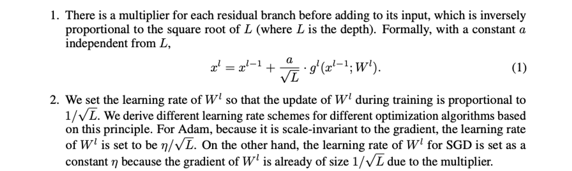
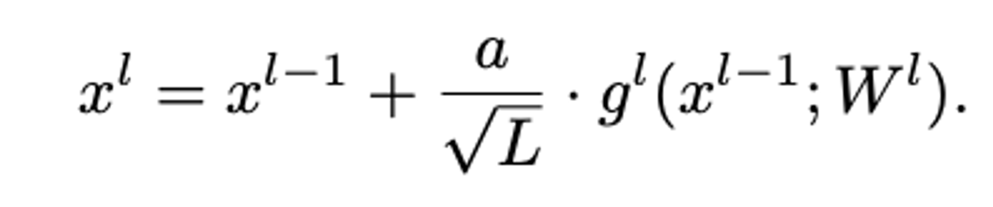
The stacking of many residual blocks causes an obvious issue even at the initialization — the norm of x l grows with l, so the last layer features do not have a stable norm when increasing the depth. Intuitively, one can stabilize these features by scaling the residual branches with a depth-dependent constant. However, scaling the residual branches with arbitrarily small constants might result in no feature learning in the large depth limit since the gradients will also be multiplied with the scaling factor

Method

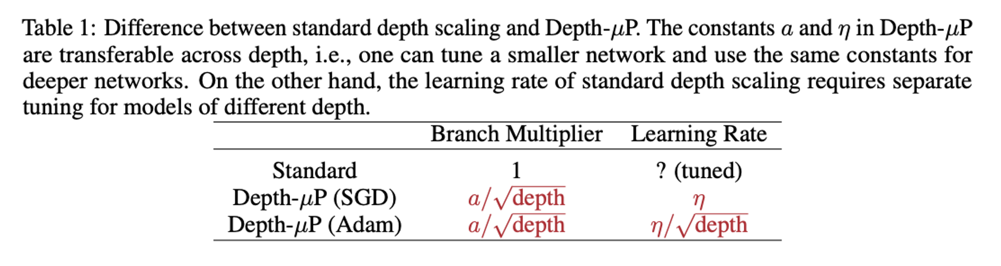
Method named “Depth-µP”

Theory demonstrates that for linear residual layers, there is a scheme that “maximizes both feature learning and feature diversity”

Also results showing in the linear case that abs scales better than relu (maximises feature diversity)

Non-linear residuals

Warm-Up

The first tricky bit here is (2). Let’s go through each term:

Fairly easy. Just the expansion imagining we had instead of . This just leaves the terms to be accounted for

The term is tricky, but made easier by the fact that the final term removes all terms, and the first term removes all terms with no s. This means we just have to sum together all the products with a single term, which is what we have here!

Removes all terms

The simplification at the end of page 5 is easy enough - just assume the shapes work and collapse the product terms

For sgd the grad formula is just the standard one where we propagate fwds and bwds.

I think the “easy to see” part below then just boils down to

(the “fact” below I think misses out a part, but this is fine as it’s just there to prove that the 1 dominates in the sum.

The final “hence” part then basically just shows that the first-order term in (2) is

I think this has two key desirable properties:

It’s not , which we’re assuming from the simplification in (2) is slamming you hard enough with the LR that you disappear (is this right?? surely at some point for a fixed LR that’s not enough?)

It doesn’t depend on depth - hence it does the same thing at different depths.

Adam is just the same except we’re missing an L term, which we make up for in the LR-scaling.

Here’s my attempt at an intuitive explanation…

Consider a fwd pass through the network after 1 update - what’s the scale of the final output?

We can answer this by looking at the network output in terms of the initial weights plus the gradient update, which itself ultimately comes from the initial weights (and activations ofc, which we assume are the same both times)

When we do this we get three terms:

The original network output before the update

Some term accounting for the effect of the update (really a summation of many terms), where each is the effect of an individual w_update on the output; never “the effect of an update’s output on the next’s update’s output” (confusing!)

We can (supposedly) ignore this w_update-w_update interaction because these updates are made small by the learning rate. When we consider this interaction we then get into territory, which we can just ignore

The focus is then on this second term (the “feature update”). We want to make sure it

Doesn’t change with depth

Isn’t in territory

To analyse the second term we need to expand out the grad_w part of it. This is just the standard grad formula where we propagate fwds and bwds, hitting all the weights except the one we update (also multiplying by the terms we added - this comes back later)

This ofc is just like the maths in the rest of the second term (the non-grad_w part)! So much so that we basically end up just squaring what we had before, and multiplying by our initial activation and loss terms (which we can ignore)

We now need to consider the depth-scaling of this residual-block product. This turns out to be easy because of the term we added (this is why it’s necessary!). It ends up that each term is simply dominated by the 1, and we have L of the terms.

This then just boils down to (in their version everything is squared, but otherwise similar)

However, this gets multiplied by a factor now in the grad_w term, and again by another factor in the original (2) formulation. This cancels with the above to make that term

Tada! We’ve satisfied out two criteria above. This is the maximal update as it matches big theta - if it was little o I think we’d not be maximal, any more though and we’d explode.

Key assumption: ignore multiplicative update effects

Results

Linear models

Top row → linear residual model has depth-µP

Middle row → compromise setup

Bottom row → SP is poor!

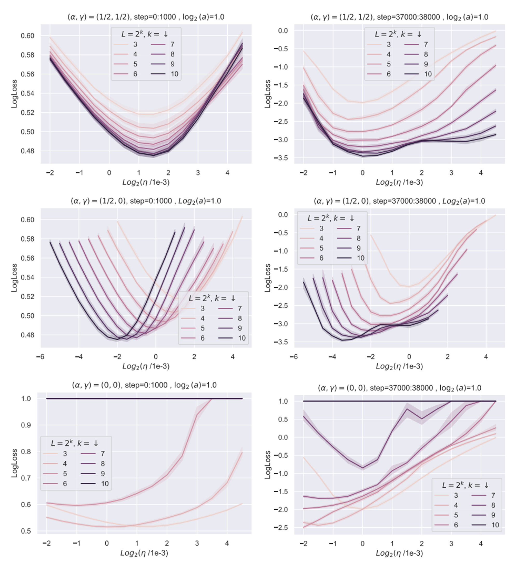
Note that in their framework feature diversity is key. Below is the ODE parameterization which is also a feature learning limit, but doesn’t maximise feature diversity. We can see it’s doesn’t quite obey µP.

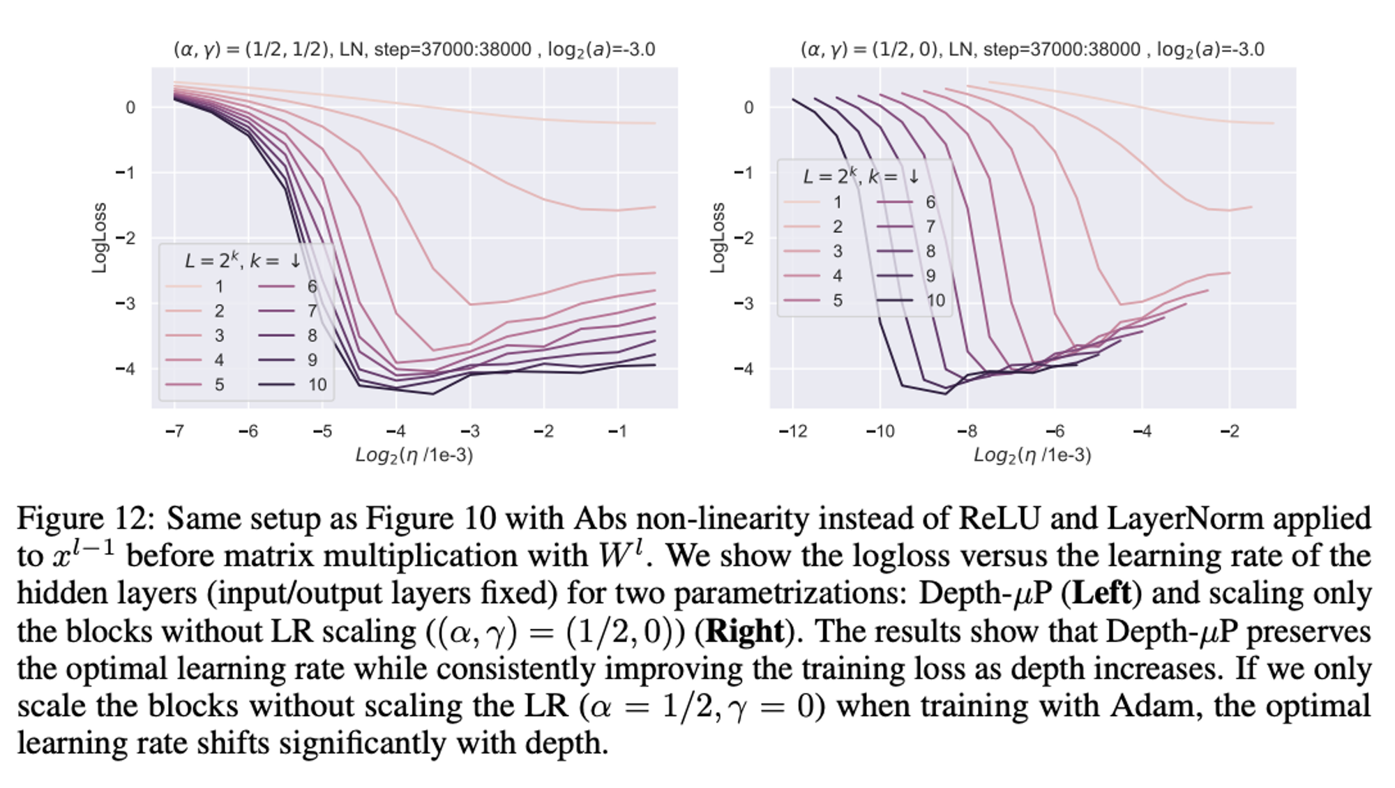
When they switch to using layernorm and abs, things get a bit messier. They still claim this obeys muP, but I’m not convinced

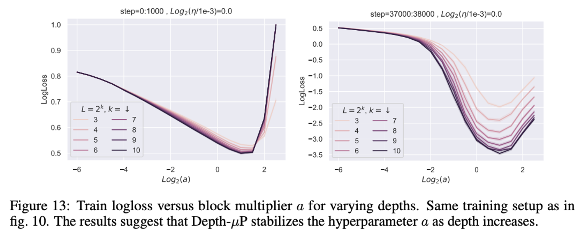
The block multiplier hyperparam also seems to be stable.

Transformers

Transformers don’t have consistent depth scaling with the given rule (as expected, given the theory is shown not to hold for them.

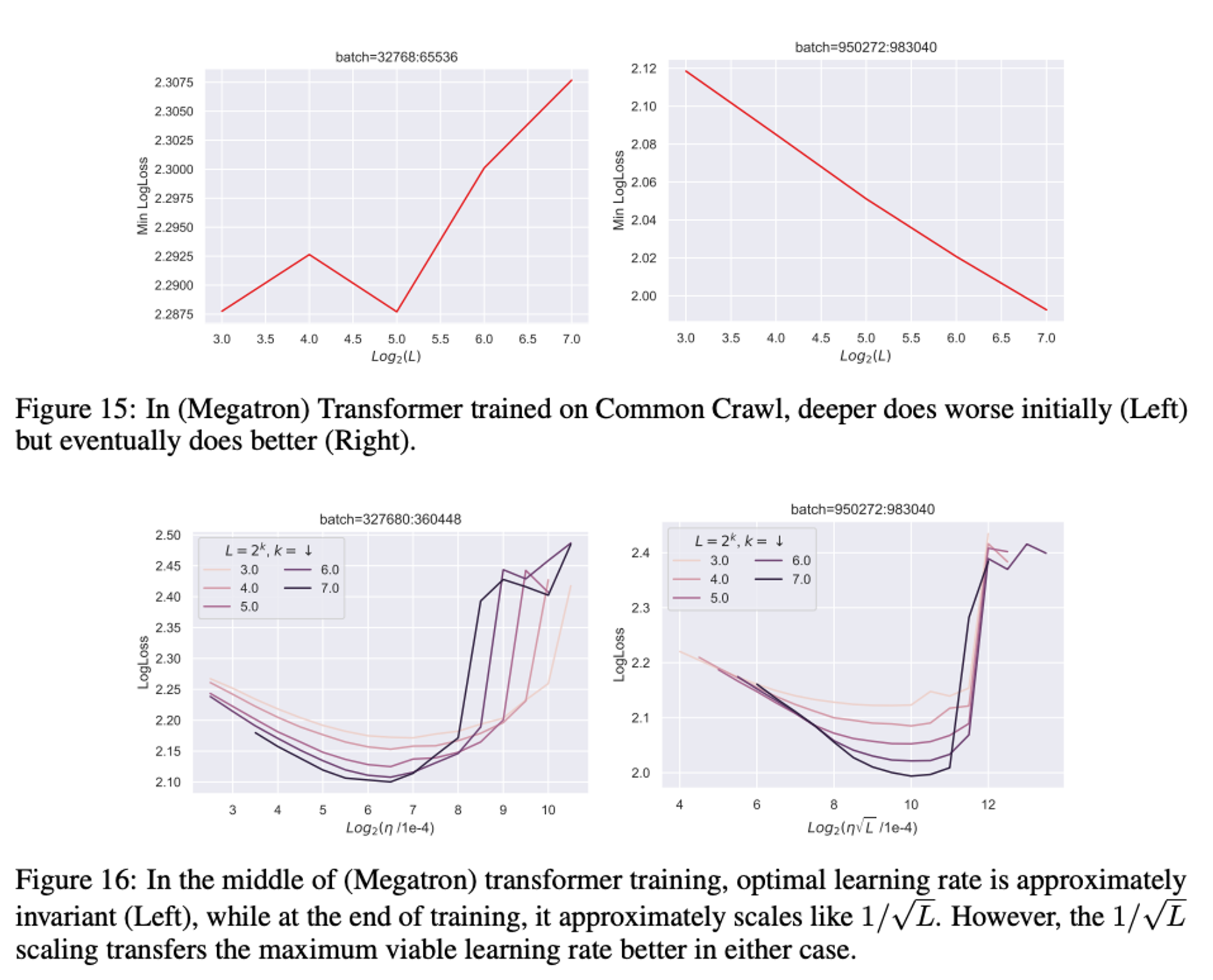
(not sure what to make of the top plots?)

Key point: the bottom plots have different x-axis scales!

The message here seems to be that at different points in training, different scaling is appropriate. They generally recommend the scaling if you have to pick one.

My instinct here is that we only care about the end of training anyway, so surely if we get the right plot after having trained we’re ok!? Maybe the fact that this doesn’t hold throughout training though is a sufficient red flag to suggest we should be cautious…

I guess a key issue is that the best LR may no longer be independent of training time - but was that ever the case?? Perhaps we’re now more sensitive to it though

this leads us to conclude that while the 1/√L scaling can potentially be practically useful in transformer training, it is likely to be brittle to architectural and algorithmic changes, or even simple things like training time

Open questions

They complain in the introduction:

The stacking of many residual blocks causes an obvious issue even at the initialization — the norm of x l grows with l, so the last layer features do not have a stable norm when increasing the depth.

But does that not happen to them too?

Surely at the first iteration of this is larger than because we’ve added a term to this without scaling the part down in the summation??

Answer? I guess the point is that yes, it does increase the scale here, but perhaps by an amount which doesn’t change as you increase depth. This would be simple if every residual took , but in this case it’s a bit more tricky. I guess this is where the adjusted learning rate comes-in, although it’s still the same for each tensor.

Overall I think I still instinctively like running-mean more than this.